3.2.5. Inversion Input File

The lines of input file for maginv3d_60.exe are as follows:

Line #	Description	Description
1	Inversion mode	1 or 2
2	Beta parameter and tolerance	par tol
3	Observations file	path to observations file
4	Sensitivity matrix	path to sensitivity (.mtx) file
5	Initial model	initial model
6	Reference model	reference model
7	Active model	sets active cells in inversion
8	Upper bounds	upper bounds for cells
9	Lower bounds	lower bounds for cells
10	alpha_s alpha_x alpha_y alpha_z	weighting constants for smallness and smoothness constraints
11	Hard constraints	SMOOTH_MOD or SMOOTH_MOD_DIF
12	Additional weights	add additional weights to cells or faces
13	Set compact and blocky norms	Set compact and blocky norms
14	Compact and blocky norm scaling	scale eps epsGrad
15	MOF derivatives	Set as null for the time-being

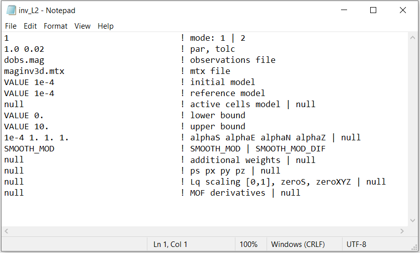
An example of the input file for L2 inversion is shown below. You may also Download the input file for a sparse norm inversion .

Fig. 3.4 Example input file for the inversion (Download ).

3.2.5.1. Line Descriptions

• Inversion mode: An integer specifying one of two choices for determining the trade-off parameter.

  • 1 - the program chooses the trade off parameter by carrying out a line search so that the target value of data misfit is achieved (e.g. \(\phi^*_d = N\))

  • 2 - the user inputs the trade off parameter.

• Beta parameter and tolerance: Two real numbers par and tol that depend upon the value on Line 1.

  • If inversion mode = 1, the target misfit value is given by the product of par and the number of data \(N\) , i.e., par=1 is equivalent to \(\phi_d^*=N\) and par=0.5 is equivalent to \(\phi_d^*=N/2\) . The second parameter, tol, is the misfit tolerance in fractional percentage. The target misfit is considered to be achieved when the relative difference between the true and target misfits is less than tolc. Normally, par=1 is ideal if the true standard deviation of error is assigned to each datum. When tol=0, the program assumes a default value of tol=0.02 since this number must be positive.

  • If inversion mode = 2, par is the value of the trade off parameter. In this case, tol is not used by the program.

• Observations file: filepath to the observations file

• Sensitivity matrix: filepath to the binary file containing the sensitivity matrix.

• Initial model: The initial susceptibility model (SI) can be defined as a value for uniform models (e.g. VALUE 0.001), or by a filename. The initial model must be within the upper and lower bounds.

• Reference model: The reference susceptibility model (SI) can be defined as a value for uniform models (e.g. VALUE 0), or by a filename (for non-uniform reference models).

• Active cells: Use the flag null if all cells below the surface topography are active in the inversion. Or provide the filepath to an active model file to define the active cells.

• Lower bound:

  • Use the flag null for no lower bound.

  • Use the flag VALUE followed by a numeric value to apply the same lower bound to all cells

  • Enter the filepath to a model file to set individual lower bounds to each cell

• Upper bound:

  • Use the flag null for no upper bound.

  • Use the flag VALUE followed by a numeric value to apply the same upper bound to all cells

  • Enter the filepath to a model file to set individual upper bounds to each cell

• alpha_s alpha_x alpha_y alpha_z: Alpha parameters . Here, the user specifies the relative weighting between the smallness and smoothness component penalties on the recovered models. As a default setting, alpha_x=alpha_y=alpha_z=1 and alpha_s=1/h \(\!^2\) is suggested, where h is the average dimension of cells in the core region.

• Hard constraints: Here, the user specifies whether how the reference model is used to constrain the inversion; go to fundamentals of inversion to see how this is implemented. For the MTZTEM package:

  • use the flag SMOOTH_MOD to ignore the reference model (essential set \(m_{ref}=0\) )

  • use the flag SMOOTH_MOD_DIF to include \(m_{ref}\) in the smallness and smoothness penalty terms

• Additional weights: Name of the weights file containing weighting matrices. If null is entered, default values of unity are used (no extra weighting).

• Set compact and blocky norms:

  • For least-square inversion, use the flag null

  • For compact and blocky norms, enter the flat VALUE, followed by the Lp/Lq exponents P Qx Qy Qz. These are defined in the model objective function. The P is for the smallest model component and the Qs are for the spatial components. P, Qx, Qy and Qz must have values between 0 and 2.

• Compact and blocky norm scaling: This is ignored if null is entered on the previous line. If using compact and blocky norms, the user provide the values for paramters scale, eps and epsGrad separated by spaces.

  • scale: The scaling between Lp and Lq components in range \([0,1]\).

  • eps: is an effective zero for the model values.

  • epsGrad: is an effective zero value for the change in model values spatially (i.e., derivatives). The program will calculate these zeros based on a single standard deviation of the L2 model if null is given with no extra scaling between Lp and Lq (scale = 0.5).

• MOF derivatives: This input is currently disabled because of the upgrade to the model objective function. Use null or end the file prematurely. This could become cell-by-cell rotation model file in a future release.