Note

This example has been developed to demonstrate functionality specific to v6.0. The example can be completed using v5.0, however some functionality may not exist in v5.0 and the format of certain input files may differ slightly.

5.5. Inversion

Here the code maginv3d_v60.exe invert synthetic magntic data to recover a susceptibility model. We perform both a smooth and a sparse inversion. We use the same data that were computed in forward modeling example. Gaussian noise were added to these data with a standard deviation of 0.5 nT. Uncertainties of 0.5 nT were assigned to all data

Before running this example, you may want to do the following:

• Download and open the zip folder containing the entire mag3d example (if not done already)
• Learn how to run maginv3d_v60 and learn the format of the input files

Important

Since the sensitivities output by magsen3d_v60.exe produce a large file, we have not provided them in the zip file. You need to complete the compute sensitivities example to run the inversion.

5.5.1. Smooth Inversion

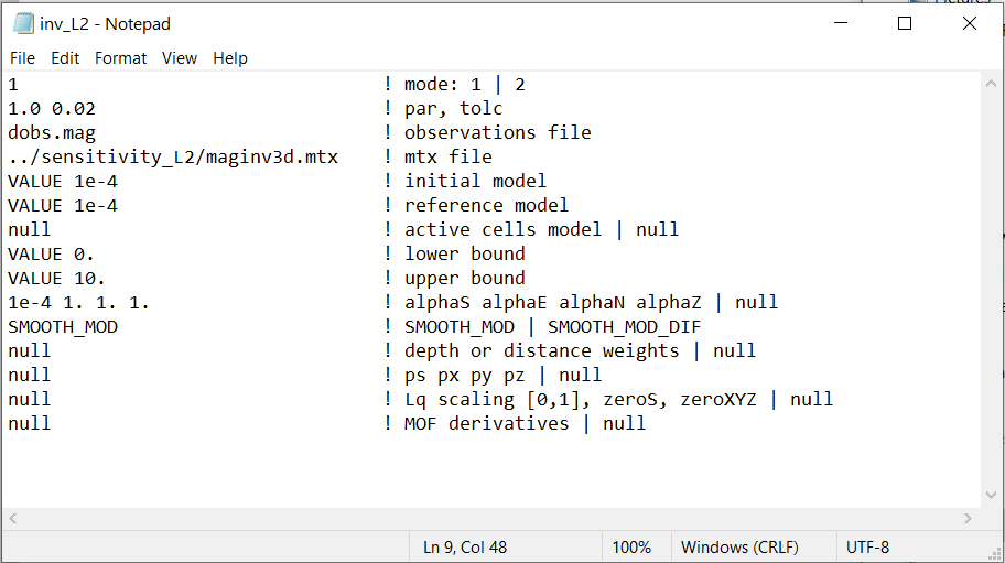
For standard L2 inversion, we use the input file inv_L2.inp and the supporting files in the sub-folder inv_L2. The input file is shown below.

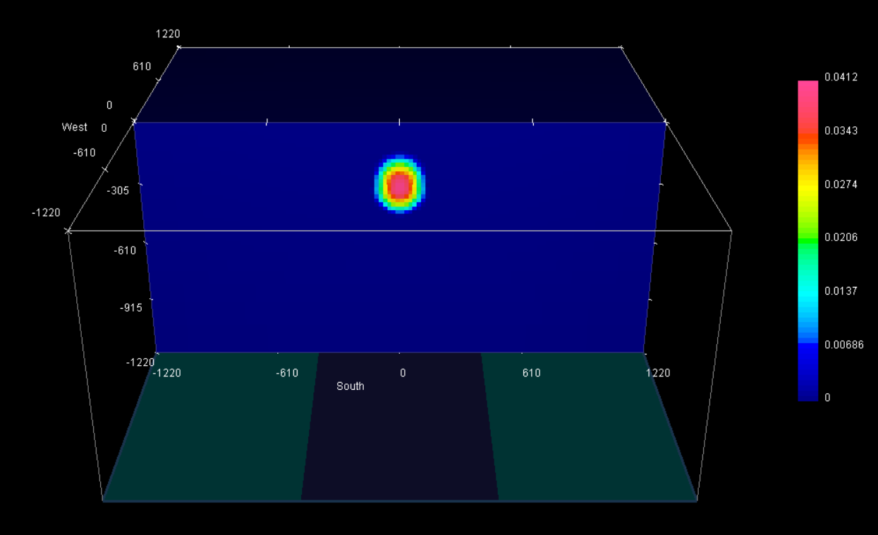
The algorithm reaches an optimum model after 5 iterations. Least-squares gravity inversion will generally place structures at the approprate locations but will underestimate the amplitude of density contrast.

5.5.2. Smooth Inversion

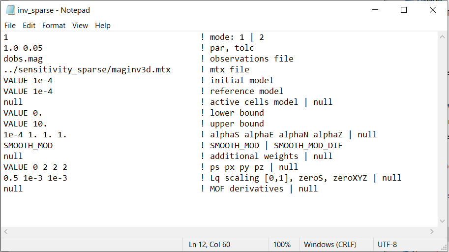
For sparse inversion, we use the input file inv_sparse.inp and the supporting files in the sub-folder inv_sparse. The input file is shown below.

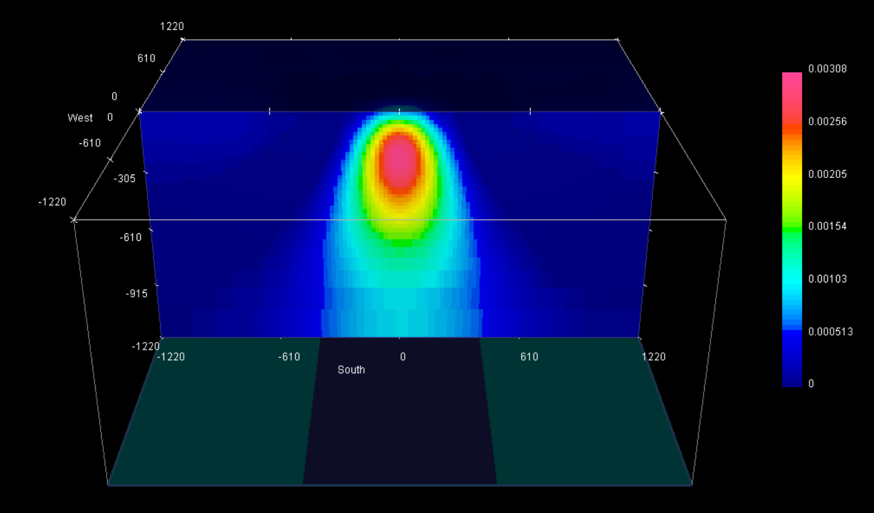
The inversion was set to recover a model that is more compact. By forcing the model to be compact, we recover a structure who density contrast of much closer to the true value of 0.1 g/cc.